在上一篇《分类任务中的类别不平衡问题(上):理论》中,我们介绍了几种常用的过采样法 (SMOTE、ADASYN 等)与欠采样法(EasyEnsemble、NearMiss 等)。正所谓“纸上得来终觉浅,绝知此事要躬行”,说了这么多,我们也该亲自上手编写代码来实践一下了。
下面我们使用之前介绍的 imbalanced-learn 库来进行实验。
准备阶段
为了方便地进行实验,我们首先通过 sklearn 提供的 make_classification 函数来构建随机数据集:
from sklearn.datasets import make_classification

def create_dataset(
    n_samples=1000,
    weights=(0.01, 0.01, 0.98),
    n_classes=3,
    class_sep=0.8,
    n_clusters=1,
):
    return make_classification(
        n_samples=n_samples,
        n_features=2,
        n_informative=2,
        n_redundant=0,
        n_repeated=0,
        n_classes=n_classes,
        n_clusters_per_class=n_clusters,
        weights=list(weights),
        class_sep=class_sep,
        random_state=0,
    )
其中,n_samples 表示样本个数,weights 表示样本的分布比例,n_classes 表示样本类别数,class_sep 表示乘以超立方体大小的因子(较大的值分散了簇/类,并使分类任务更容易),n_clusters 表示每一个类别是由几个簇构成。这里为了方便展示,我们通过 n_features=2 设定每个样本都是二维向量。
然后,为了后续直观地展示不同采样法的效果,我们运用经典的绘图库 matplotlib(以及 Seaborn)编写两个函数分别展示采样后的样本分布和分类器的决策函数(分类超平面):
import matplotlib.pyplot as plt
import seaborn as sns
import numpy as np

sns.set_context("poster")

# The following function will be used to plot the sample space after resampling
# to illustrate the specificities of an algorithm.
def plot_resampling(X, y, sampler, ax, title=None):
    X_res, y_res = sampler.fit_resample(X, y)
    ax.scatter(X_res[:, 0], X_res[:, 1], c=y_res, alpha=0.8, edgecolor="k")
    if title is None:
        title = f"Resampling with {sampler.__class__.__name__}"
    ax.set_title(title)
    sns.despine(ax=ax, offset=10)

# The following function will be used to plot the decision function of a
# classifier given some data.
def plot_decision_function(X, y, clf, ax, title=None):
    plot_step = 0.02
    x_min, x_max = X[:, 0].min() - 1, X[:, 0].max() + 1
    y_min, y_max = X[:, 1].min() - 1, X[:, 1].max() + 1
    xx, yy = np.meshgrid(
        np.arange(x_min, x_max, plot_step), np.arange(y_min, y_max, plot_step)
    )

    Z = clf.predict(np.c_[xx.ravel(), yy.ravel()])
    Z = Z.reshape(xx.shape)
    ax.contourf(xx, yy, Z, alpha=0.4)
    ax.scatter(X[:, 0], X[:, 1], alpha=0.8, c=y, edgecolor="k")
    if title is not None:
        ax.set_title(title)
其中 X, y 分别表示样本和对应的类别。特别地,plot_decision_function 函数还需要传入一个分类器,为了方便,后面所有的实验均使用 LogisticRegression 分类器:
from sklearn.linear_model import LogisticRegression

clf = LogisticRegression()
过采样法的比较
Random over-sampling
随机过采样 (Random over-sampling) 即随机地重复采样正例,imbalanced-learn 库通过 RandomOverSampler 类来实现。
在 imbalanced-learn 库中,大部分采样方法都可以使用
make_pipeline将采样方法和分类模型连接起来,但是两种集成方法 EasyEnsemble 和 BalanceCascade 无法使用make_pipeline,因为它们本质上是集成了好几个分类模型,所以需要自定义方法。
from imblearn.pipeline import make_pipeline
from imblearn.over_sampling import RandomOverSampler

X, y = create_dataset(n_samples=100, weights=(0.05, 0.25, 0.7))

fig, axs = plt.subplots(nrows=1, ncols=2, figsize=(15, 7))

clf.fit(X, y)
plot_decision_function(X, y, clf, axs[0], title="Without resampling")

sampler = RandomOverSampler(random_state=0)
model = make_pipeline(sampler, clf).fit(X, y)
plot_decision_function(X, y, model, axs[1], f"Using {model[0].__class__.__name__}")

fig.suptitle(f"Decision function of {clf.__class__.__name__}")
fig.tight_layout()
plt.show()
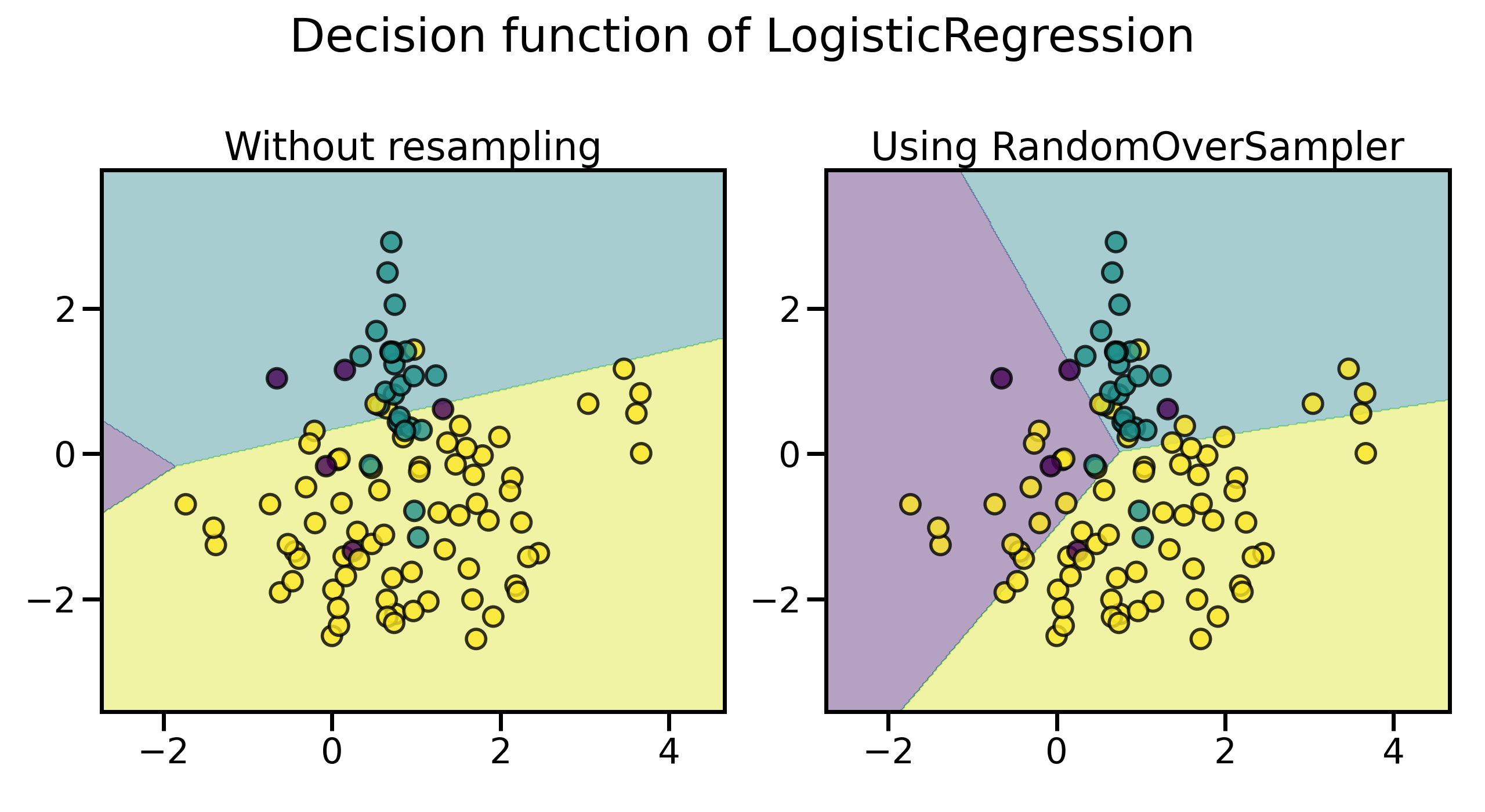
可以看到,即使通过这种最简单的方法,决策的边界也发生了明显的变化,已经较少偏向多数类了。默认情况下,随机采样生成的样本均严格地来自于原始正例集合,可以通过 shrinkage 来向采样生成的样本中添加小的扰动,从而生成一个平滑的数据集:
from imblearn.over_sampling import RandomOverSampler

X, y = create_dataset(n_samples=100, weights=(0.05, 0.25, 0.7))

sampler = RandomOverSampler(random_state=0)

fig, axs = plt.subplots(nrows=1, ncols=2, figsize=(15, 7))

sampler.set_params(shrinkage=None)
plot_resampling(X, y, sampler, ax=axs[0], title="Normal bootstrap")

sampler.set_params(shrinkage=0.3)
plot_resampling(X, y, sampler, ax=axs[1], title="Smoothed bootstrap")

fig.suptitle(f"Resampling with {sampler.__class__.__name__}")
fig.tight_layout()
plt.show()
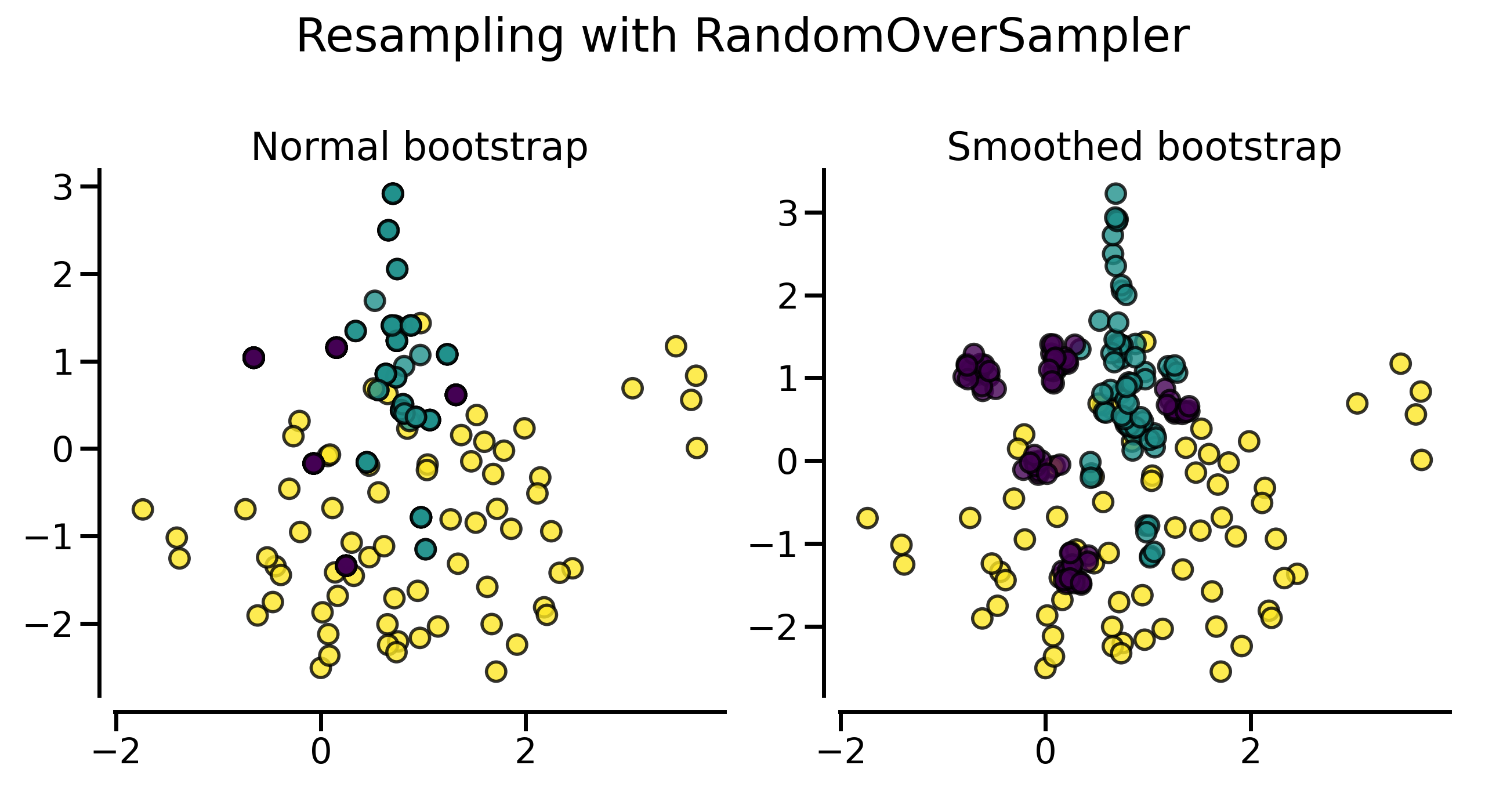
可以看到,使用平滑方式随机采样得到的数据集看上去包含了更多的样本,这实际上是因为生成的样本没有与原始样本重叠。
ADASYN 和 SMOTE
正如我们在上篇中介绍的那样,相比随机过采样会造成严重的过拟合,ADASYN 和 SMOTE 法才是更为常用的过采样法,它们不是简单地重复采样或者向生成的数据中添加扰动,而是采用一些特定的启发式方法。在 imbalanced-learn 库,它们分别通过 ADASYN 和 SMOTE 类来实现。
from imblearn import FunctionSampler  # to use a idendity sampler
from imblearn.over_sampling import RandomOverSampler
from imblearn.over_sampling import SMOTE, ADASYN

X, y = create_dataset(n_samples=150, weights=(0.1, 0.2, 0.7))

fig, axs = plt.subplots(nrows=2, ncols=2, figsize=(20, 15))

samplers = [
    FunctionSampler(),
    RandomOverSampler(random_state=0),
    SMOTE(random_state=0),
    ADASYN(random_state=0),
]

for ax, sampler in zip(axs.ravel(), samplers):
    title = "Original dataset" if isinstance(sampler, FunctionSampler) else None
    plot_resampling(X, y, sampler, ax, title=title)
fig.tight_layout()

plt.show()
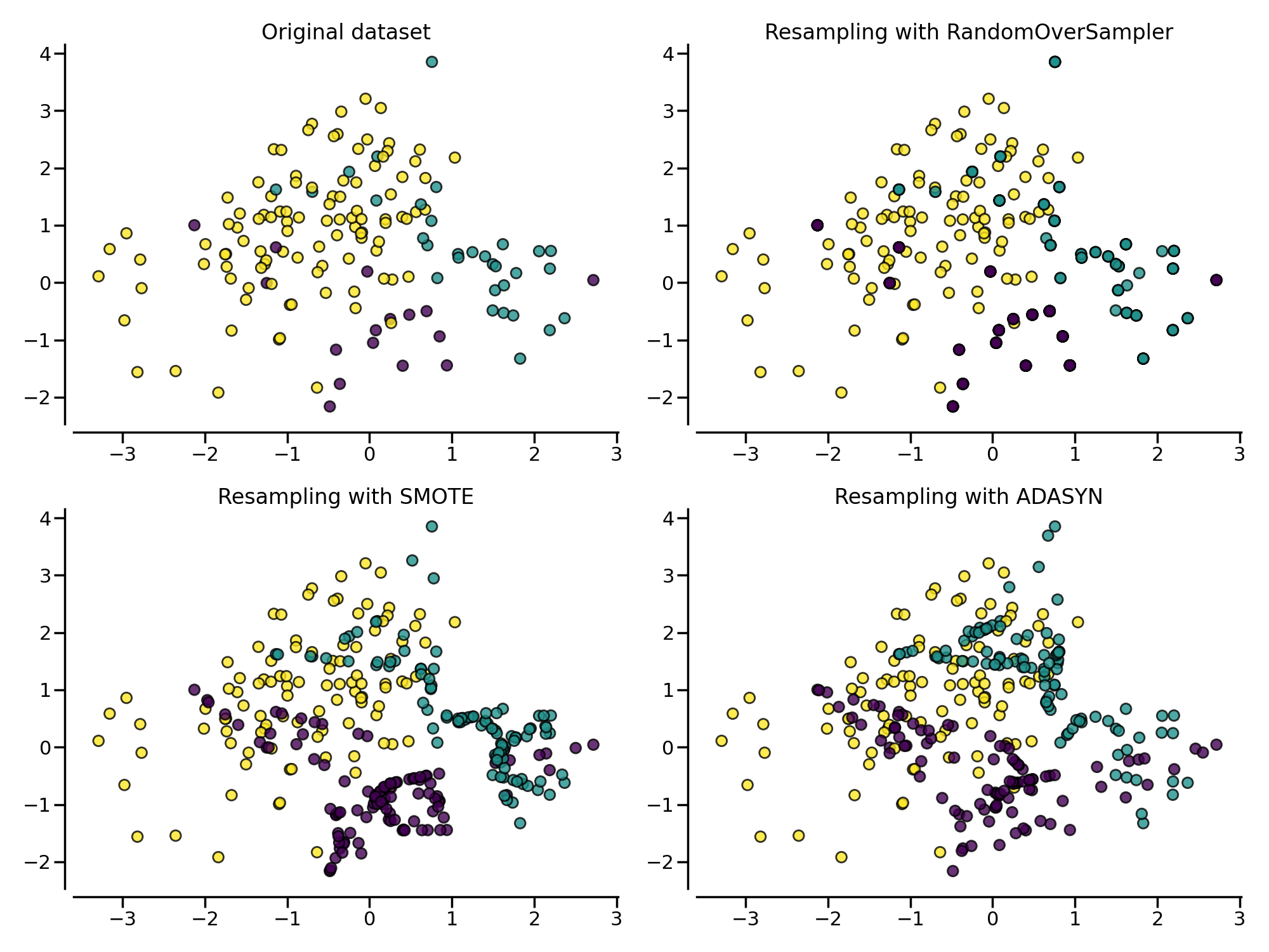
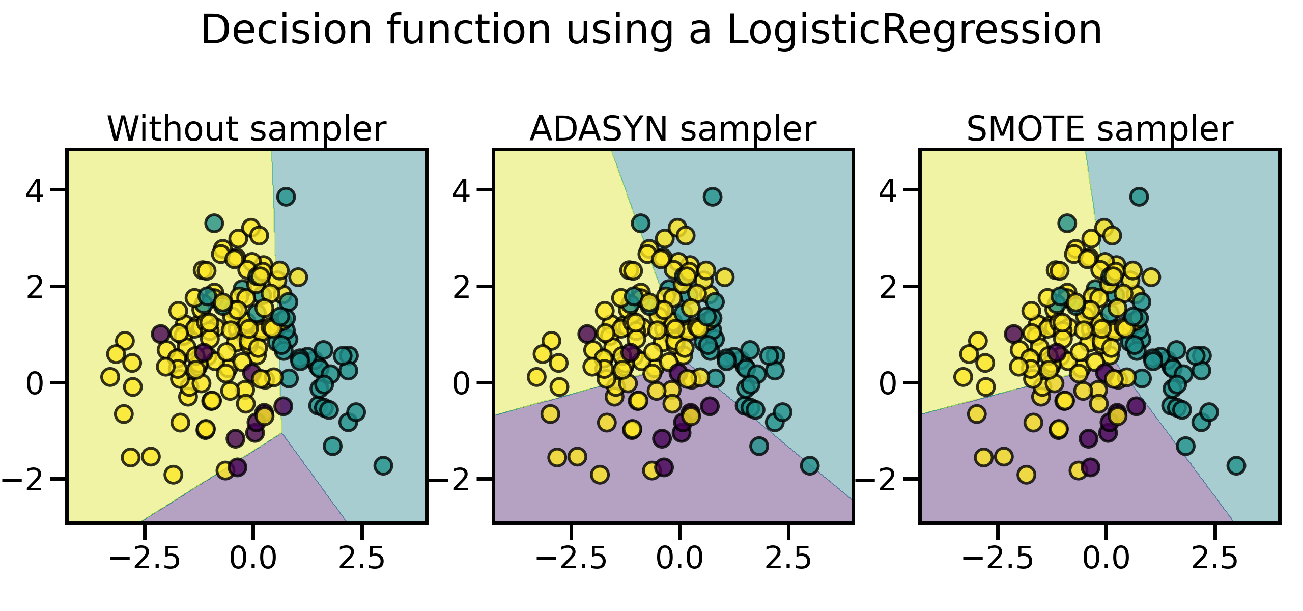
同样地,通过随机过采样法、SMOTE 和 ADASYN 得到的数据集的分类器决策函数也会不同。相比 SMOTE 法对所有正例“一视同仁”,对每个正例样本都合成相同数量的样本不同,ADASYN 法更关注那些在边界附近的正例样本(即周围的负例样本更多的正例),它们更难以通过近邻规则分类:
from imblearn.pipeline import make_pipeline
from imblearn.over_sampling import SMOTE, ADASYN

X, y = create_dataset(n_samples=150, weights=(0.05, 0.25, 0.7))

fig, axs = plt.subplots(nrows=1, ncols=3, figsize=(20, 6))

models = {
    "Without sampler": clf,
    "ADASYN sampler": make_pipeline(ADASYN(random_state=0), clf),
    "SMOTE sampler": make_pipeline(SMOTE(random_state=0), clf),
}

for ax, (title, model) in zip(axs, models.items()):
    model.fit(X, y)
    plot_decision_function(X, y, model, ax=ax, title=title)

fig.suptitle(f"Decision function using a {clf.__class__.__name__}")
fig.tight_layout()

plt.show()
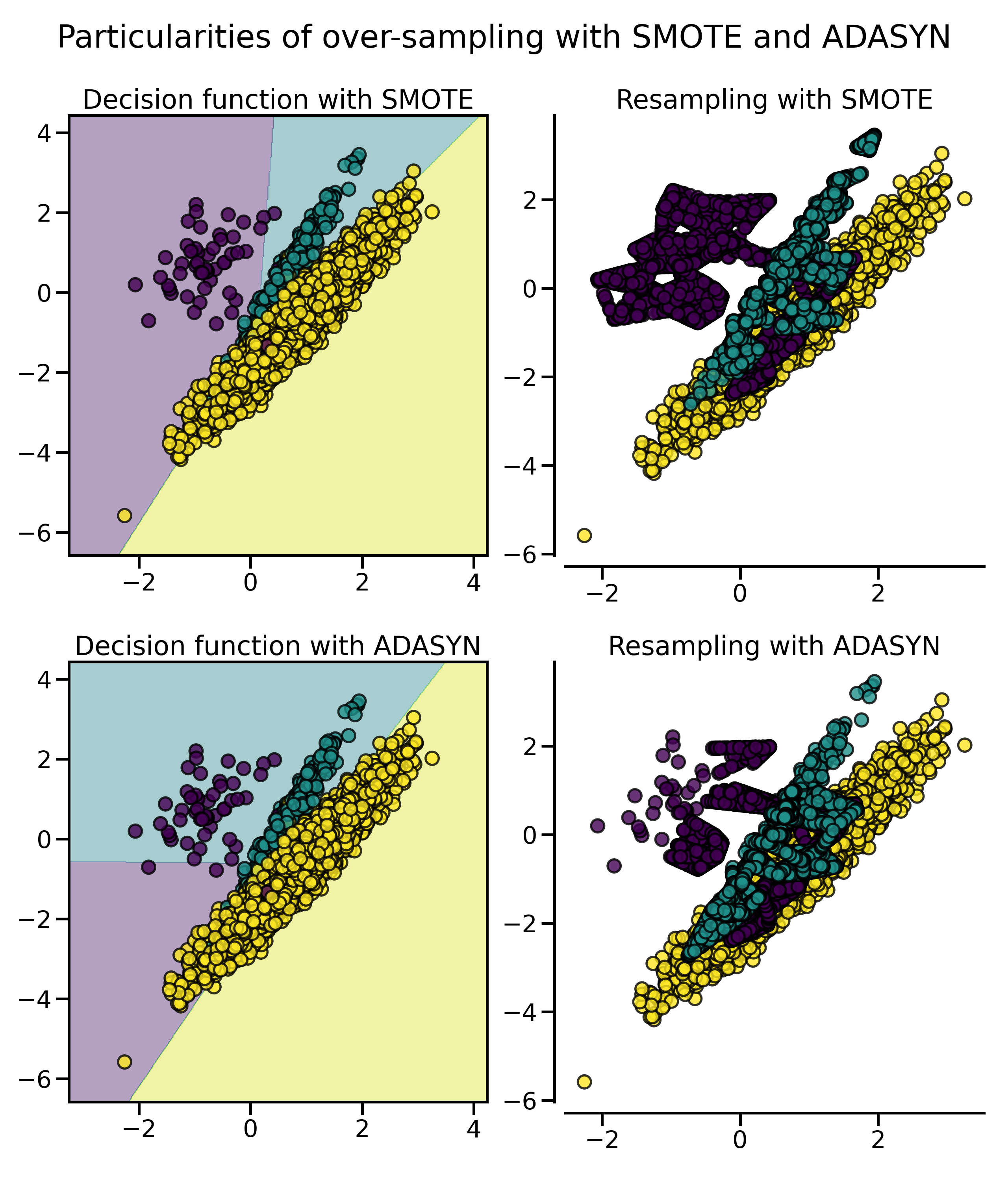
尤其是在样本比较多的情况下,这两种采样法的特性会更加明显,用 SMOTE 合成的样本分布比较平均,而 ADASYN 生成的样本大都来自于原来与负例比较靠近的那些正例样本,它们也可能会引起一些问题:
from imblearn.pipeline import make_pipeline
from imblearn.over_sampling import SMOTE, ADASYN

X, y = create_dataset(n_samples=5000, weights=(0.01, 0.05, 0.94), class_sep=0.8)

samplers = [SMOTE(random_state=0), ADASYN(random_state=0)]

fig, axs = plt.subplots(nrows=2, ncols=2, figsize=(15, 15))
for ax, sampler in zip(axs, samplers):
    model = make_pipeline(sampler, clf).fit(X, y)
    plot_decision_function(
        X, y, clf, ax[0], title=f"Decision function with {sampler.__class__.__name__}"
    )
    plot_resampling(X, y, sampler, ax[1])

fig.suptitle("Particularities of over-sampling with SMOTE and ADASYN")
fig.tight_layout()

plt.show()
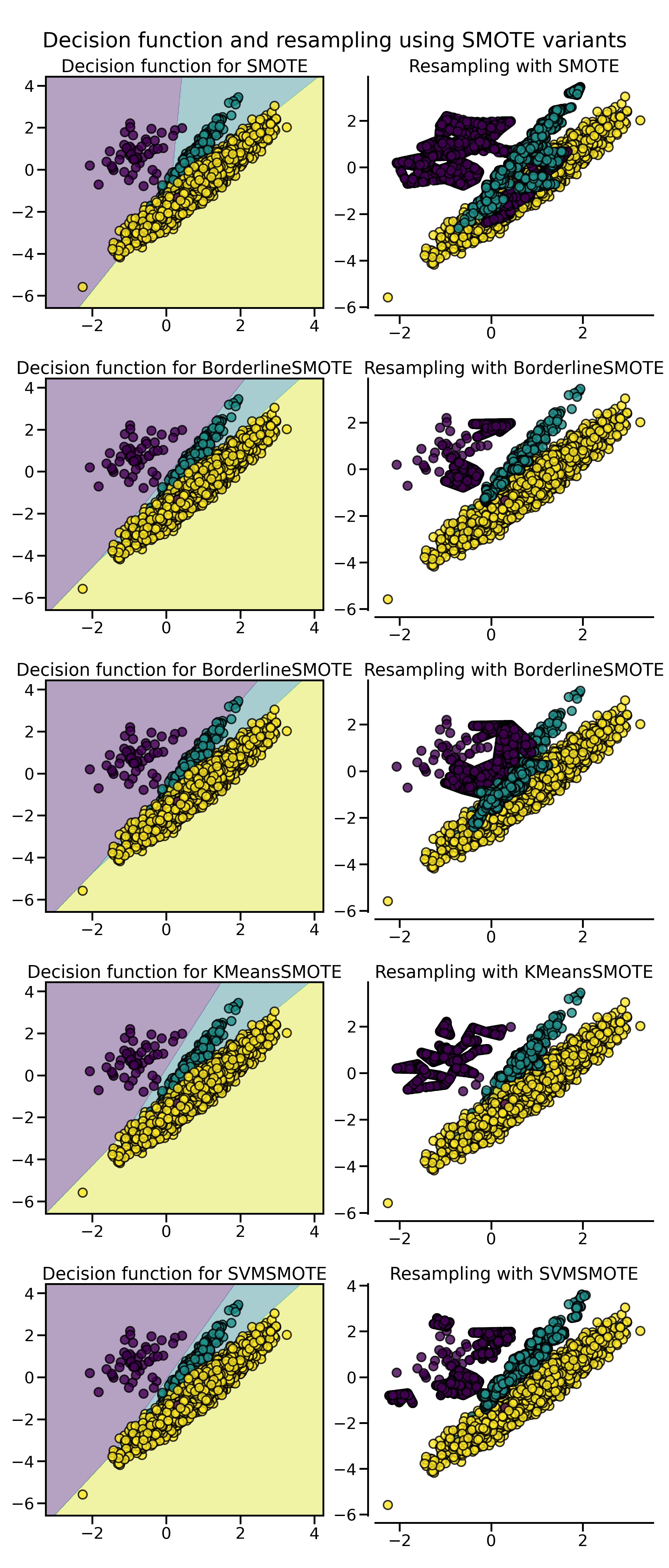
正如我们在上篇中介绍的那样,SMOTE 算法根据对正例样本的选择还有一些变体,例如 Border-line SMOTE 会选择那些在边界上的正例。除此以外,常用的还有
- 使用 SVM 的支持向量来生成新样本的 SVMSMOTE;
- 先进行聚类,然后根据聚类密度在每个聚类中独立生成样本。
在 imbalanced-learn 库,它们分别通过 BorderlineSMOTE、KMeansSMOTE 和 SVMSMOTE 类来实现。
from imblearn.pipeline import make_pipeline
from imblearn.over_sampling import SMOTE, BorderlineSMOTE, KMeansSMOTE, SVMSMOTE

X, y = create_dataset(n_samples=5000, weights=(0.01, 0.05, 0.94), class_sep=0.8)

fig, axs = plt.subplots(5, 2, figsize=(15, 30))

samplers = [
    SMOTE(random_state=0),
    BorderlineSMOTE(random_state=0, kind="borderline-1"),
    BorderlineSMOTE(random_state=0, kind="borderline-2"),
    KMeansSMOTE(random_state=0),
    SVMSMOTE(random_state=0),
]

for ax, sampler in zip(axs, samplers):
    model = make_pipeline(sampler, clf).fit(X, y)
    plot_decision_function(
        X, y, clf, ax[0], title=f"Decision function for {sampler.__class__.__name__}"
    )
    plot_resampling(X, y, sampler, ax[1])

fig.suptitle("Decision function and resampling using SMOTE variants")
fig.tight_layout()

plt.show()
混合特征与离散特征
在某些情况下,样本同时包含了连续和离散特征(混合特征),这时只能使用 SMOTENC 法来处理。例如,我们构建一个模拟数据集,样本包含三个维度,其中第 1、3 维为离散特征,第 2 维为连续特征:
from collections import Counter
from imblearn.over_sampling import SMOTENC

rng = np.random.RandomState(42)
n_samples = 50
# Create a dataset of a mix of numerical and categorical data
X = np.empty((n_samples, 3), dtype=object)
X[:, 0] = rng.choice(["A", "B", "C"], size=n_samples).astype(object)
X[:, 1] = rng.randn(n_samples)
X[:, 2] = rng.randint(3, size=n_samples)
y = np.array([0] * 20 + [1] * 30)

print("The original imbalanced dataset")
print(sorted(Counter(y).items()))
print()
print("The first and last columns are containing categorical features:")
print(X[:5])
print()

smote_nc = SMOTENC(categorical_features=[0, 2], random_state=0)
X_resampled, y_resampled = smote_nc.fit_resample(X, y)
print("Dataset after resampling:")
print(sorted(Counter(y_resampled).items()))
print()
print("SMOTE-NC will generate categories for the categorical features:")
print(X_resampled[-5:])
print()
The original imbalanced dataset
[(0, 20), (1, 30)]

The first and last columns are containing categorical features:
[['C' -0.14021849735700803 2]
 ['A' -0.033193400066544886 2]
 ['C' -0.7490765234433554 1]
 ['C' -0.7783820070908942 2]
 ['A' 0.948842857719016 2]]

Dataset after resampling:
[(0, 30), (1, 30)]

SMOTE-NC will generate categories for the categorical features:
[['A' 0.5246469549655818 2]
 ['B' -0.3657680728116921 2]
 ['B' 0.9344237230779993 2]
 ['B' 0.3710891618824609 2]
 ['B' 0.3327240726719727 2]]
可以看到,只需要通过 categorical_features 参数指定离散特征的维度,SMOTENC 采样法就可以生成同时包含离散和连续特征的样本,使得数据集类别平衡。但是,如果数据集只包含离散特征,那么应该直接使用 SMOTEN 过采样法:
from collections import Counter
from imblearn.over_sampling import SMOTEN

# Generate only categorical data
X = np.array(["A"] * 10 + ["B"] * 20 + ["C"] * 30, dtype=object).reshape(-1, 1)
y = np.array([0] * 20 + [1] * 40, dtype=np.int32)

print(f"Original class counts: {Counter(y)}")
print()
print(X[:5])
print()

sampler = SMOTEN(random_state=0)
X_res, y_res = sampler.fit_resample(X, y)
print(f"Class counts after resampling {Counter(y_res)}")
print()
print(X_res[-5:])
print()
Original class counts: Counter({1: 40, 0: 20})

[['A']
 ['A']
 ['A']
 ['A']
 ['A']]

Class counts after resampling Counter({0: 40, 1: 40})

[['B']
 ['B']
 ['A']
 ['B']
 ['A']]
欠采样法的比较
欠采样法大致可以分为两类:可控欠采样法 (controlled under-sampling)和数据清洗方法 (leaning under-sampling)。对于可控欠采样法来说,采样的负例样本数是可以被预先设定的,例如最简单的随机欠采样。
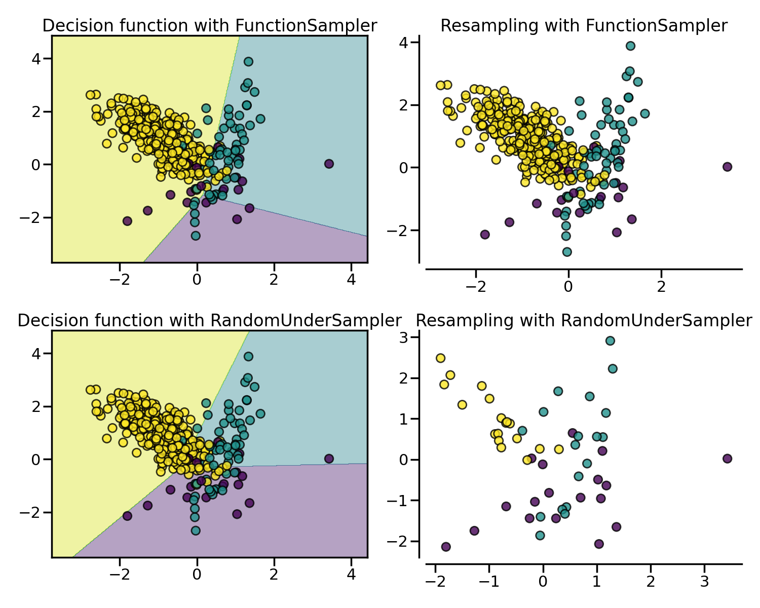
Random under-sampling
随机欠采样法 (Random under-sampling) 思想非常简单,即随机地从负例集合中采样指定数量的样本。imbalanced-learn 库通过 RandomUnderSampler 类来实现。
from imblearn import FunctionSampler
from imblearn.pipeline import make_pipeline
from imblearn.under_sampling import RandomUnderSampler

X, y = create_dataset(n_samples=400, weights=(0.05, 0.15, 0.8), class_sep=0.8)

samplers = {
    FunctionSampler(),  # identity resampler
    RandomUnderSampler(random_state=0),
}

fig, axs = plt.subplots(nrows=2, ncols=2, figsize=(15, 12))
for ax, sampler in zip(axs, samplers):
    model = make_pipeline(sampler, clf).fit(X, y)
    plot_decision_function(
        X, y, model, ax[0], title=f"Decision function with {sampler.__class__.__name__}"
    )
    plot_resampling(X, y, sampler, ax[1])

fig.tight_layout()

plt.show()
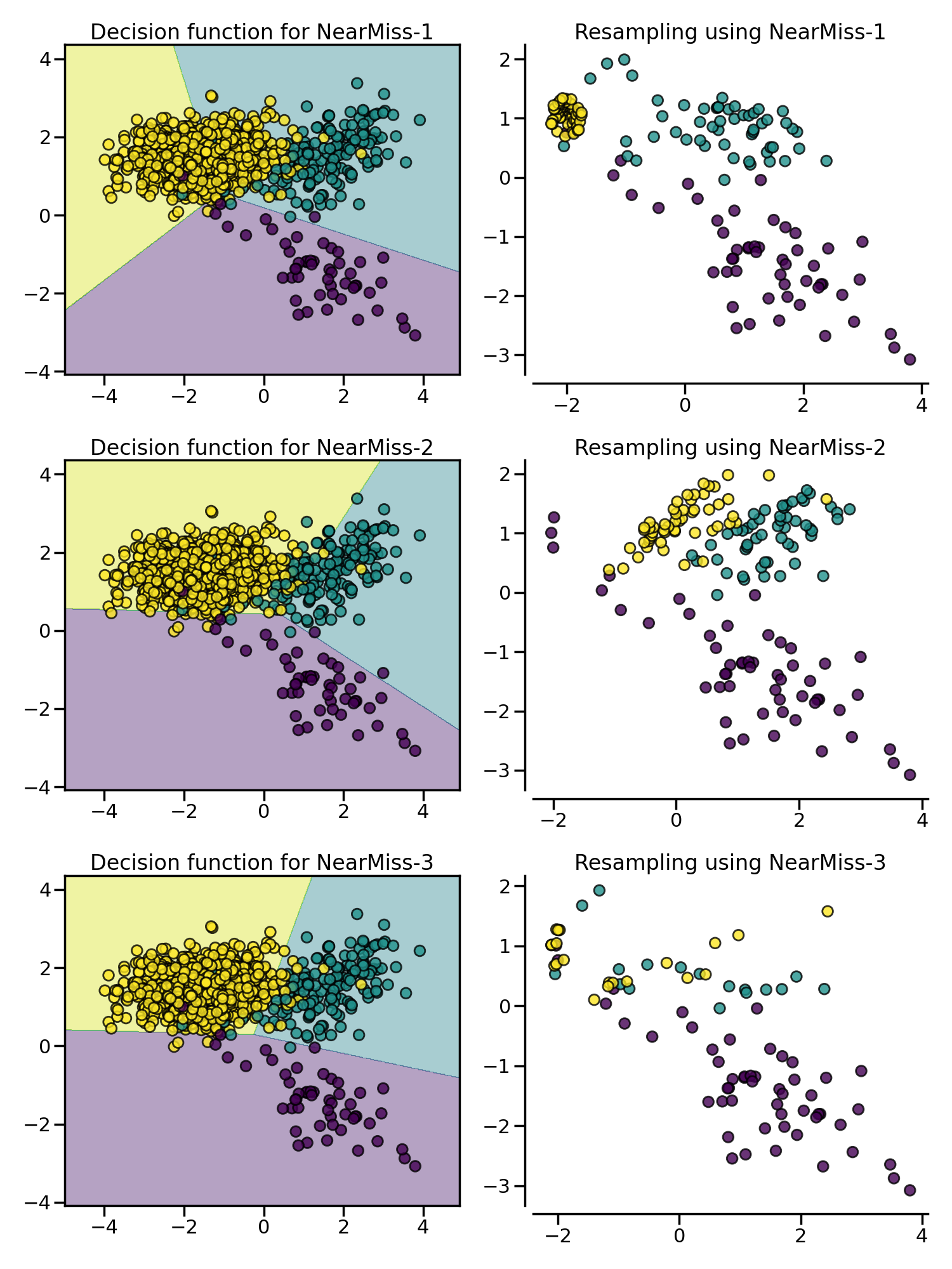
NearMiss
NearMiss 采样法通过一些启发式的规则来选择负例:NearMiss-1 选择到最近的 $K$ 个正例样本平均距离最近的负例样本;NearMiss-2 选择到最远的 $K$ 个正例样本平均距离最近的负例样本;NearMiss-3 则是一个两阶段算法,首先对于每一个正例样本,它们的 $m$ 个最近的邻居会被保留,然后选择那些与 $K$ 个最近邻的平均距离最大的负例样本。
from imblearn.pipeline import make_pipeline
from imblearn.under_sampling import NearMiss

X, y = create_dataset(n_samples=1000, weights=(0.05, 0.15, 0.8), class_sep=1.5)

samplers = [NearMiss(version=1), NearMiss(version=2), NearMiss(version=3)]

fig, axs = plt.subplots(nrows=3, ncols=2, figsize=(15, 20))
for ax, sampler in zip(axs, samplers):
    model = make_pipeline(sampler, clf).fit(X, y)
    plot_decision_function(
        X, y, model, ax[0],
        title=f"Decision function for {sampler.__class__.__name__}-{sampler.version}",
    )
    plot_resampling(
        X, y, sampler, ax[1],
        title=f"Resampling using {sampler.__class__.__name__}-{sampler.version}",
    )
fig.tight_layout()
数据清洗方法
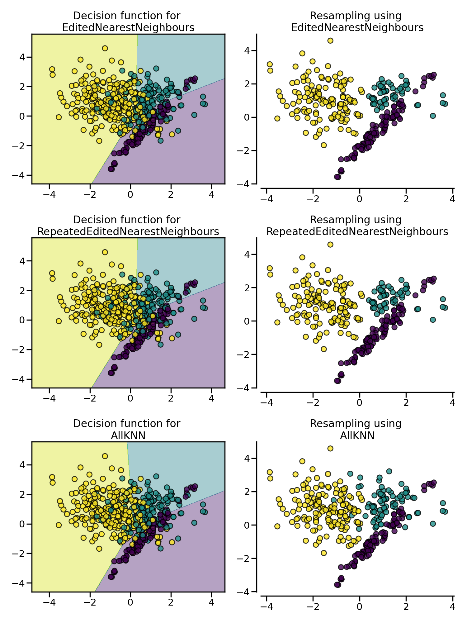
Edited Nearest Neighbours (ENN)
Edited Nearest Neighbours (ENN) 欠采样法删除那些与其最近的邻居之一不同的负例样本,并且这个过程可以不断重复,称为 Repeated Edited Nearest Neighbours。与 Repeated Edited Nearest Neighbours 法在内部最近邻算法采用固定的 $K$ 不同,AllKNN 法采取可变的 $K$ 参数,并且在每次迭代时增加 $K$。
from imblearn.pipeline import make_pipeline
from imblearn.under_sampling import (
    EditedNearestNeighbours,
    RepeatedEditedNearestNeighbours,
    AllKNN,
)

X, y = create_dataset(n_samples=500, weights=(0.2, 0.3, 0.5), class_sep=0.8)

samplers = [
    EditedNearestNeighbours(),
    RepeatedEditedNearestNeighbours(),
    AllKNN(allow_minority=True),
]

fig, axs = plt.subplots(3, 2, figsize=(15, 20))
for ax, sampler in zip(axs, samplers):
    model = make_pipeline(sampler, clf).fit(X, y)
    plot_decision_function(
        X, y, clf, ax[0], title=f"Decision function for \n{sampler.__class__.__name__}"
    )
    plot_resampling(
        X, y, sampler, ax[1], title=f"Resampling using \n{sampler.__class__.__name__}"
    )

fig.tight_layout()

plt.show()
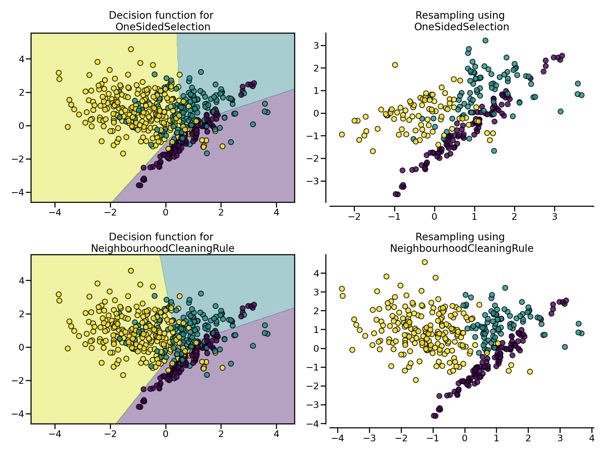
Tomek Link
Tomek Link 表示不同类别之间距离最近的一对样本,即两个样本互为最近邻且分属不同类别,通过移除 Tomek Link 就能“清洗掉”类间重叠样本,使得互为最近邻的样本皆属于同一类别。imbalanced-learn 库通过 OneSidedSelection 类来实现。类似的还有 NeighbourhoodCleaningRule 算法,它通过 Edited Nearest Neighbours 来移除负例样本。
from imblearn.pipeline import make_pipeline
from imblearn.under_sampling import (
    OneSidedSelection,
    NeighbourhoodCleaningRule,
)

X, y = create_dataset(n_samples=500, weights=(0.2, 0.3, 0.5), class_sep=0.8)

fig, axs = plt.subplots(nrows=2, ncols=2, figsize=(20, 15))

samplers = [
    OneSidedSelection(random_state=0),
    NeighbourhoodCleaningRule(),
]

for ax, sampler in zip(axs, samplers):
    model = make_pipeline(sampler, clf).fit(X, y)
    plot_decision_function(
        X, y, clf, ax[0], title=f"Decision function for \n{sampler.__class__.__name__}"
    )
    plot_resampling(
        X, y, sampler, ax[1], title=f"Resampling using \n{sampler.__class__.__name__}"
    )
fig.tight_layout()

plt.show()
集成学习方法
在上篇中我们也介绍过,EasyEnsemble 和 BalanceCascade 采用集成学习机制来处理随机欠采样中的信息丢失问题。在集成分类器中,bagging 方法在不同的随机选择的数据子集上构建多个估计器,scikit-learn 中采用 BaggingClassifier 类来实现。 但是,它不会平衡每个数据子集,因此将偏向于多数类:
from sklearn.datasets import make_classification
from sklearn.model_selection import train_test_split
from sklearn.metrics import balanced_accuracy_score
from sklearn.ensemble import BaggingClassifier
from sklearn.tree import DecisionTreeClassifier

X, y = make_classification(n_samples=10000, n_features=2, n_informative=2,
                           n_redundant=0, n_repeated=0, n_classes=3,
                           n_clusters_per_class=1,
                           weights=[0.01, 0.05, 0.94],
                           class_sep=0.8, random_state=0)
X_train, X_test, y_train, y_test = train_test_split(X, y, random_state=0)

bc = BaggingClassifier(base_estimator=DecisionTreeClassifier(), random_state=0)
bc.fit(X_train, y_train)
y_pred = bc.predict(X_test)
print(balanced_accuracy_score(y_test, y_pred))
0.7739629664028289
很显然,可以通过前面介绍的采样方法来平衡每个数据子集,scikit-learn 中采用 BalancedBaggingClassifier 类来实现。采样由 sampler 或者 sampling_strategy 和 replacement 这两个参数控制,例如使用随机欠采样 (Random under-sampling):
from imblearn.ensemble import BalancedBaggingClassifier
bbc = BalancedBaggingClassifier(base_estimator=DecisionTreeClassifier(),
                                sampling_strategy='auto',
                                replacement=False,
                                random_state=0)
bbc.fit(X_train, y_train)
y_pred = bbc.predict(X_test)
print(balanced_accuracy_score(y_test, y_pred))
0.8251353587264241
可以看到在经过采样使得数据集平衡后,分类的准确率得到了提升。
EasyEnsemble 法可以理解为使用 AdaBoostClassifier 作为学习器的特定 bagging 方法,它允许对在平衡 bootstrap 样本上训练的 AdaBoost 学习器进行打包。与 BalancedBaggingClassifier 的用法相似,scikit-learn 中采用 EasyEnsembleClassifier 类来实现:
from imblearn.ensemble import EasyEnsembleClassifier
eec = EasyEnsembleClassifier(random_state=0)
eec.fit(X_train, y_train)
y_pred = eec.predict(X_test)
print(balanced_accuracy_score(y_test, y_pred))
0.6248477859302602
结合过采样和欠采样
我们之前已经说过,SMOTE 算法的问题是可能会在边缘异常值和内部值之间插入新点,从而生成噪声样本,而这个问题可以通过清理过采样产生的空间来解决,即将二者结合起来,先过采样再进行数据清洗。常用的方法是 SMOTE + Edited Nearest Neighbours (ENN) 和 SMOTE + Tomek Link,在 imbalanced-learn 库分别通过 SMOTEENN 和 SMOTETomek 类来实现:
from imblearn.pipeline import make_pipeline
from imblearn import FunctionSampler
from imblearn.over_sampling import SMOTE
from imblearn.combine import SMOTEENN, SMOTETomek

X, y = make_classification(n_samples=5000, n_features=2, n_informative=2,
                           n_redundant=0, n_repeated=0, n_classes=3,
                           n_clusters_per_class=1,
                           weights=[0.01, 0.05, 0.94],
                           class_sep=0.8, random_state=0)

fig, axs = plt.subplots(4, 2, figsize=(15, 25))

samplers = [
    FunctionSampler(),
    SMOTE(random_state=0),
    SMOTEENN(random_state=0),
    SMOTETomek(random_state=0)
]

for ax, sampler in zip(axs, samplers):
    model = make_pipeline(sampler, clf).fit(X, y)
    plot_decision_function(
        X, y, clf, ax[0], title=f"Decision function for {sampler.__class__.__name__}"
    )
    plot_resampling(X, y, sampler, ax[1])

fig.tight_layout()

plt.show()
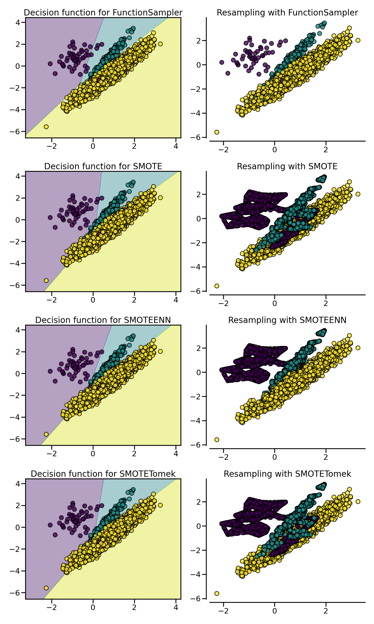
可以看到,相比于 SMOTE + Tomek Link 法,SMOTE + Edited Nearest Neighbours (ENN) 通常能清除更多的噪声样本。
参考
[1] 机器学习之类别不平衡问题 (3) —— 采样方法
[2] imbalanced-learn 库 User Guide