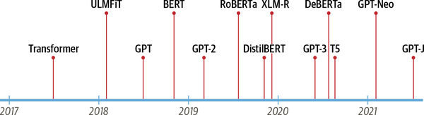
自从 2017 年 Google 发布《Attention is All You Need》之后,各种基于 Transformer 的模型和方法层出不穷。2018 年,OpenAI 发布的 Generative Pretrained Transformer (GPT) 和 Google 发布的 Bidirectional Encoder Representations from Transformers (BERT) 模型在几乎所有 NLP 任务上都取得了远超先前 SOTA 基准的性能,将 Transformer 模型的热度推上了新的高峰。
目前大部分的研究者都直接使用封装好的深度学习包来进行实验(例如适用于 PyTorch 框架的 Transformers,以及适用于 Keras 框架的 bert4keras),这固然很方便,但是并不利于深入理解模型结构,尤其是对于 NLP 研究领域的入门者。
本文从介绍模型结构出发,使用 Pytorch 框架,手把手地带大家实现一个 Transformer block。
Transformer 结构
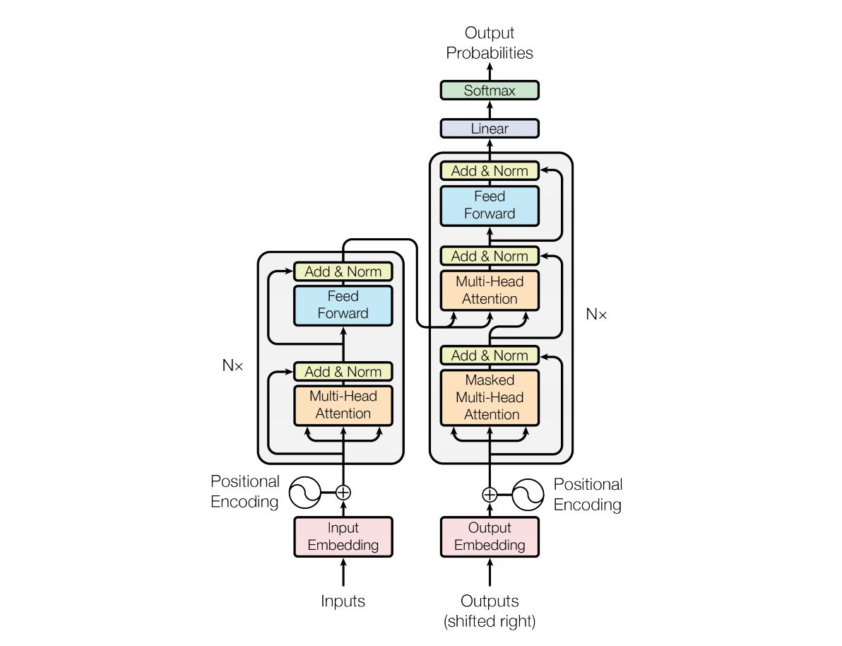
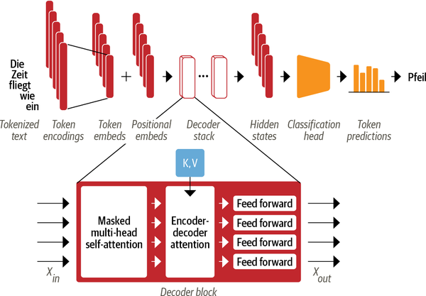
标准的 Transformer 模型采用 Encoder-Decoder 框架,如下图所示,Encoder 负责将输入的 token 序列转换为嵌入式向量序列(又称隐状态或上下文),Decoder 则基于 Encoder 的隐状态来迭代地生成一个 token 序列作为输出,每次生成一个 token。
其中,Encoder 和 Decoder 都各自包含有多个 building blocks,下图展示了一个翻译任务的例子:
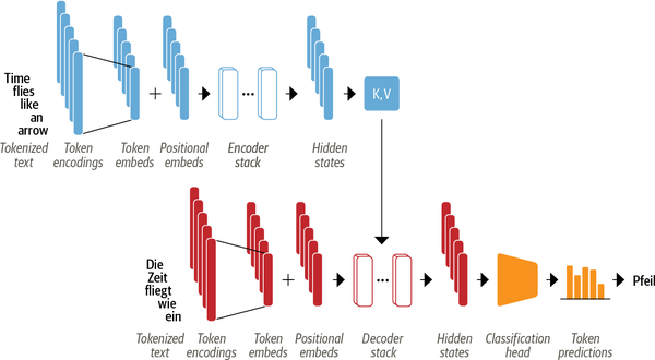
可以看到:
- 输入的 token 首先被转换为嵌入向量 token embeddings。由于注意力机制无法捕获 token 之间的位置关系,因此还通过 positional embeddings 向输入中添加位置信息来建模文本的词语顺序;
- Encoder 由一堆 encoder layers (blocks) 组成,类似于图像领域中的堆叠卷积层。同样地,在 Decoder 中也包含有堆叠的 decoder layers;
- Encoder 的输出被送入到 Decoder 层中以预测概率最大的下一个 token,然后当前步骤生成的 token 序列又被送回到 Decoder 中以继续生成下一个 token。重复这一过程,直到出现序列结束符 EOS 或者超过最大输出长度。
虽然 Transformer 最初是设计用于完成 Seq2Seq 任务的,但是其中的 Encoder 和 Decoder blocks 也都可以单独使用。因此,无论 Transformer 模型如何变化,都可以归纳为下面的三种类型:
纯 Encoder:将输入文本转换为嵌入式表示,适用于处理文本分类和命名实体识别等任务。BERT 以及它的变体(例如 RoBERTa/DistilBERT)就属于该类型。该框架根据每一个 token 前后的上下文来生成对应的嵌入式表示,也被称为双向注意力 (Bidirectional Attention)。
纯 Decoder:给定一个模板 (prompt),例如“Thanks for lunch, I had a…”,这个类型的模型就可以通过迭代地预测概率最大的下一个词来自动补全序列。GPT 模型家族就属于该类型。该框架下每一个 token 的嵌入式表示只依赖于 token 左侧的上下文,因此也被称为因果/自回归注意力 (causal/autoregressive attention)。
Encoder-Decoder:用于建模从一个序列文本到另一个的复杂映射,适用于机器翻译和文本摘要等任务。BART 和 T5 就属于该类型。
纯 Encoder 和纯 Decoder 模型的界限很多时候是模糊的,例如纯 Decoder 的 GPT 模型也可以用于完成序列到序列的翻译任务,而纯 Encoder 的 BERT 模型也可以用于处理通常由 Encoder-Decoder 和纯 Decoder 模型完成的摘要任务。
Attention
各种 NLP 神经网络模型的本质就是对文本(token 序列)进行编码,常规的做法是首先将每个 token 都转化为对应的词向量 (token embeddings),将文本转换为一个矩阵 $\boldsymbol{X} = (\boldsymbol{x}_1, \boldsymbol{x}_2, …, \boldsymbol{x}_n)$,其中 $\boldsymbol{x}_i$ 就表示第 $i$ 个 token 的 embedding。
在 Transformer 模型提出之前,对 token 序列 $\boldsymbol{X}$ 的常规编码方式是通过循环网络 (RNNs) 和卷积网络 (CNNs)。
-
RNN(例如 LSTM)的方案很简单,每一个词语 $\boldsymbol{x}_t$ 对应的编码结果 $\boldsymbol{y}_t$ 通过递归地计算得到:
\[\boldsymbol{y}_t =f(\boldsymbol{y}_{t-1},\boldsymbol{x}_t) \tag{1}\]RNN 虽然建模方式与人类阅读类似,但是其最大缺点是无法并行计算,因此速度较慢,而且还难以处理远距离的词语交互;
-
CNN 则通过滑动窗口基于局部上下文来编码文本,例如核尺寸为 3 的卷积操作就是使用每一个 token 自身以及其前一个和后一个 token 来生成嵌入式表示:
\[\boldsymbol{y}_t = f(\boldsymbol{x}_{t-1},\boldsymbol{x}_t,\boldsymbol{x}_{t+1}) \tag{2}\]CNN 能够并行地计算,但是因为是通过窗口来进行编码,所以更侧重于捕获局部信息,难以建模长距离的语义依赖。
《Attention is All You Need》提供了第三个方案:直接使用 Attention 机制编码整个文本。相比 RNN 要逐步递归才能获得全局信息(因此一般使用双向 RNN),而 CNN 实际只能获取局部信息,需要通过层叠来增大感受野,Attention 机制一步到位获取了全局信息:
\[\boldsymbol{y}_t = f(\boldsymbol{x}_t,\boldsymbol{A},\boldsymbol{B}) \tag{3}\]其中 $\boldsymbol{A},\boldsymbol{B}$ 是另外的 token 序列(矩阵),如果取 $\boldsymbol{A}=\boldsymbol{B}=\boldsymbol{X}$,那么就称为 Self-Attention,即直接将 $\boldsymbol{x}_t$ 与自身序列中的每个 token 进行比较,最后算出 $\boldsymbol{y}_t$。
Scaled Dot-product Attention
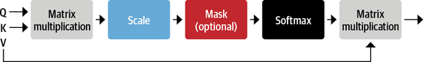
虽然 Attention 有许多种实现方式,但是最常见的是 Scaled Dot-product Attention,共包含 2 个主要步骤:
-
计算注意力权重:使用某种相似度函数来度量每一个 query 向量和所有 key 向量之间的关联程度。Scaled Dot-product Attention 使用点积作为相似度函数,这样相似的 queries 和 keys 具有较大的点积。对于序列长度为 $m$ 的 Query 序列和长度为 $n$ 的 Key 序列,该步骤会生成一个尺寸为 $m \times n$ 的注意力分数矩阵。
点积可以产生任意大的数字,这会破坏训练过程的稳定性。因此注意力分数还需要乘以一个缩放因子来标准化它们的方差,然后用一个 softmax 标准化。这样就得到了最终的注意力权重 $w_{ij}$,表示第 $i$ 个 query 向量与第 $j$ 个 key 向量之间的关联程度。
-
更新 token embeddings:将权重 $w_{ij}$ 与对应的 value 向量 $\boldsymbol{v}_1,…,\boldsymbol{v}_n$ 相乘以获得第 $i$ 个 query 向量更新后的语义表示 $\boldsymbol{x}_i’ = \sum_{j} w_{ij}\boldsymbol{v}_j$。
形式化表示为:
\[\text{Attention}(\boldsymbol{Q},\boldsymbol{K},\boldsymbol{V}) = \text{softmax}\left(\frac{\boldsymbol{Q}\boldsymbol{K}^{\top}}{\sqrt{d_k}}\right)\boldsymbol{V} \tag{4}\]其中 $\boldsymbol{Q}\in\mathbb{R}^{m\times d_k}, \boldsymbol{K}\in\mathbb{R}^{n\times d_k}, \boldsymbol{V}\in\mathbb{R}^{n\times d_v}$ 是 query、key、value 向量序列。如果忽略 softmax 激活函数,实际上它就是三个 $m\times d_k,d_k\times n, n\times d_v$ 矩阵相乘,得到一个 $m\times d_v$ 的矩阵,也就是将 $m\times d_k$ 的序列 $\boldsymbol{Q}$ 编码成了一个新的 $m\times d_v$ 的序列。
将上面的公式拆开来看更加清楚:
\[\text{Attention}(\boldsymbol{q}_t,\boldsymbol{K},\boldsymbol{V}) = \sum_{s=1}^m \frac{1}{Z}\exp\left(\frac{\langle\boldsymbol{q}_t, \boldsymbol{k}_s\rangle}{\sqrt{d_k}}\right)\boldsymbol{v}_s \tag{5}\]其中 $Z$ 是归一化因子。$\boldsymbol{K},\boldsymbol{V}$ 是一一对应的 key 和 value 向量序列,Scaled Dot-product Attention 就是通过 $\boldsymbol{q}_t$ 这个 query 与各个 $\boldsymbol{k}_s$ 内积的并 softmax 的方式,来得到 $\boldsymbol{q}_t$ 与各个 $\boldsymbol{v}_s$ 的相似度,然后加权求和,得到一个 $d_v$ 维的向量。其中因子 $\sqrt{d_k}$ 起到调节作用,使得内积不至于太大。
下面我们通过手工实现 Scaled Dot-product Attention 来更详细地了解这一过程:
首先,我们需要通过分词将文本转换为 token 序列,然后将每一个 token 转换为对应的 embedding。在 Pytorch 中,我们可以通过 torch.nn.Embedding 层来完成该操作,相当于构建一个从 token ID 到 token embedding 的 映射表:
from torch import nn
from transformers import AutoConfig
from transformers import AutoTokenizer

model_ckpt = "bert-base-uncased"
tokenizer = AutoTokenizer.from_pretrained(model_ckpt)

text = "time flies like an arrow"
inputs = tokenizer(text, return_tensors="pt", add_special_tokens=False)
print(inputs.input_ids)

config = AutoConfig.from_pretrained(model_ckpt)
token_emb = nn.Embedding(config.vocab_size, config.hidden_size)
print(token_emb)

inputs_embeds = token_emb(inputs.input_ids)
print(inputs_embeds.size())
tensor([[ 2051, 10029,  2066,  2019,  8612]])
Embedding(30522, 768)
torch.Size([1, 5, 768])
为了演示方便,这里我们通过
add_special_tokens=False去除了分词结果中的[CLS]和[SEP]。
可以看到,BERT-base 模型对应的词表大小为 30522,每个 token 的 embedding 维度为 768。通过映射表我们把输入的 token 序列映射为了一个尺寸为 [batch_size, seq_len, hidden_dim] 的张量。这样接下来就是创建 query、key 和 value 向量序列,并且使用点积作为相似度函数来计算注意力分数:
import torch
from math import sqrt

query = key = value = inputs_embeds
dim_k = key.size(-1)
scores = torch.bmm(query, key.transpose(1,2)) / sqrt(dim_k)
print(scores.size())
torch.Size([1, 5, 5])
可以看到我们为序列长度为 5 的样本创建了一个 $5\times 5$ 的注意力分数矩阵,并且按嵌入向量的大小进行了缩放。接下来,就是应用 softmax 标准化注意力权重:
import torch.nn.functional as F

weights = F.softmax(scores, dim=-1)
print(weights.sum(dim=-1))
tensor([[1., 1., 1., 1., 1.]], grad_fn=<SumBackward1>)
最后就是将注意力权重与 value 序列相乘:
attn_outputs = torch.bmm(weights, value)
print(attn_outputs.shape)
torch.Size([1, 5, 768])
至此我们已经实现了一个简化版的 Scaled Dot-product Attention。我们将上面这些操作封装为函数以方便后续调用:
import torch
import torch.nn.functional as F
from math import sqrt

def scaled_dot_product_attention(query, key, value, query_mask=None, key_mask=None, mask=None):
    dim_k = query.size(-1)
    scores = torch.bmm(query, key.transpose(1, 2)) / sqrt(dim_k)
    if query_mask is not None and key_mask is not None:
        mask = torch.bmm(query_mask.unsqueeze(-1), key_mask.unsqueeze(1))
    if mask is not None:
        scores = scores.masked_fill(mask == 0, -float("inf"))
    weights = F.softmax(scores, dim=-1)
    return torch.bmm(weights, value)
上面的代码还考虑了 query、key、value 序列的 Mask。padding 的字符不应该参与计算,因此将对应的注意力分数设置为 -inf,这样 softmax 之后 其对应的注意力权重就为 0 了($e^{-\infty}=0$)。
但是 Scaled Dot-product Attention 的最大问题是,当 query 和 key 序列相同时,注意力机制会为上下文中的相同单词分配非常大的分数(点积为 1)。但在实践中,上下文中的相关词往往比相同词更重要,例如只有引入上下文中“time”和“arrow”这些词的信息才能够确认“flies”的含义。
因此,Multi-head Attention 出现了!它首先通过三个不同的线性映射将 query、key 和 value 序列映射到三个不同的特征空间,然后在映射后的序列上应用 Scaled Dot-product Attention,并且把这个过程重复做多次。
Multi-head Attention
Multi-headed Attention 将每一组线性投影后的向量表示视为一个头 (head),然后在每一组表示上都应用 Scaled Dot-product Attention,也就是计算多个注意力头,如下图所示:
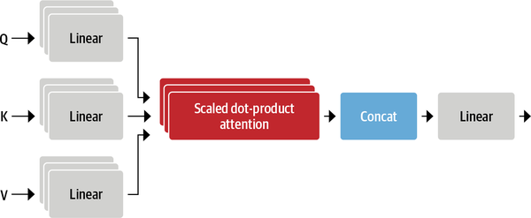
由于每个注意力头只倾向于关注某一方面的语义相似性,所以多个头可以让模型同时关注多个方面。例如,一个注意力头可以专注于捕获主谓交互,而另一个头则可以找到附近的形容词。因此,与简单的 Scaled Dot-product Attention 相比,Multi-head Attention 可以捕获到更加复杂的特征信息。
形式化表示为:
\[\begin{gather}head_i = \text{Attention}(\boldsymbol{Q}\boldsymbol{W}_i^Q,\boldsymbol{K}\boldsymbol{W}_i^K,\boldsymbol{V}\boldsymbol{W}_i^V)\\\text{MultiHead}(\boldsymbol{Q},\boldsymbol{K},\boldsymbol{V}) = \text{Concat}(head_1,...,head_h)\end{gather} \tag{6}\]其中 $\boldsymbol{W}_i^Q\in\mathbb{R}^{d_k\times \tilde{d}_k}, \boldsymbol{W}_i^K\in\mathbb{R}^{d_k\times \tilde{d}_k}, \boldsymbol{W}_i^V\in\mathbb{R}^{d_v\times \tilde{d}_v}$ 是映射矩阵,$h$ 是注意力头的数量。最后,我们将多头的结果拼接起来就得到最终 $m\times h\tilde{d}_v$ 的编码结果序列。所谓的“多头” (Multi-head),其实就是多做几次 Scaled Dot-product Attention(参数不共享),然后把结果拼接。
因此,Multi-head Attention 的结构实际并不复杂,下面我们首先实现一个注意力头:
from torch import nn

class AttentionHead(nn.Module):
    def __init__(self, embed_dim, head_dim):
        super().__init__()
        self.q = nn.Linear(embed_dim, head_dim)
        self.k = nn.Linear(embed_dim, head_dim)
        self.v = nn.Linear(embed_dim, head_dim)

    def forward(self, query, key, value, query_mask=None, key_mask=None, mask=None):
        attn_outputs = scaled_dot_product_attention(
            self.q(query), self.k(key), self.v(value), query_mask, key_mask, mask)
        return attn_outputs
可以看到,我们初始化了三个独立的线性层,通过对 query、key、value 序列应用矩阵乘法来生成尺寸为 [batch_size, seq_len, head_dim] 的张量,其中 head_dim 是我们映射到的向量维度。实践中我们一般将 head_dim 设置为 embed_dim 的倍数,这样 token 嵌入式表示的维度就可以保持不变,例如 BERT 有 12 个注意力头,因此每个头的维度被设置为 $768 / 12 = 64$。
下面我们拼接多个注意力头的输出以构建完整的 Multi-head Attention 层:
class MultiHeadAttention(nn.Module):
    def __init__(self, config):
        super().__init__()
        embed_dim = config.hidden_size
        num_heads = config.num_attention_heads
        head_dim = embed_dim // num_heads
        self.heads = nn.ModuleList(
            [AttentionHead(embed_dim, head_dim) for _ in range(num_heads)]
        )
        self.output_linear = nn.Linear(embed_dim, embed_dim)

    def forward(self, query, key, value, query_mask=None, key_mask=None, mask=None):
        x = torch.cat([
            h(query, key, value, query_mask, key_mask, mask) for h in self.heads
        ], dim=-1)
        x = self.output_linear(x)
        return x
这里我们将多个注意力头的输出拼接后,再通过一个线性变换来生成最终的输出张量。
我们使用预训练 BERT 的参数初始化 Multi-head Attention 层,并且将前面构建的输入送入模型以验证模型是否符合我们的预期:
from transformers import AutoConfig
from transformers import AutoTokenizer

model_ckpt = "bert-base-uncased"
tokenizer = AutoTokenizer.from_pretrained(model_ckpt)

text = "time flies like an arrow"
inputs = tokenizer(text, return_tensors="pt", add_special_tokens=False)
config = AutoConfig.from_pretrained(model_ckpt)
token_emb = nn.Embedding(config.vocab_size, config.hidden_size)
inputs_embeds = token_emb(inputs.input_ids)

multihead_attn = MultiHeadAttention(config)
query = key = value = inputs_embeds
attn_output = multihead_attn(query, key, value)
print(attn_output.size())
torch.Size([1, 5, 768])
Transformer Encoder
The Feed-Forward Layer
Transformer Encoder/Decoder 中的前馈子层实际上就是简单的两层全连接神经网络,它单独地处理序列中的每一个嵌入向量,因此也被称为 position-wise feed-forward layer。基于经验的做法是让第一层的维度是嵌入向量大小的 4 倍,然后以 GELU 作为激活函数。
下面我们基于 nn.Module 实现一个简单的 Feed-Forward Layer:
class FeedForward(nn.Module):
    def __init__(self, config):
        super().__init__()
        self.linear_1 = nn.Linear(config.hidden_size, config.intermediate_size)
        self.linear_2 = nn.Linear(config.intermediate_size, config.hidden_size)
        self.gelu = nn.GELU()
        self.dropout = nn.Dropout(config.hidden_dropout_prob)

    def forward(self, x):
        x = self.linear_1(x)
        x = self.gelu(x)
        x = self.linear_2(x)
        x = self.dropout(x)
        return x
我们将前面注意力层的输出送入到该层中以测试是否符合我们的预期:
feed_forward = FeedForward(config)
ff_outputs = feed_forward(attn_output)
print(ff_outputs.size())
torch.Size([1, 5, 768])
至此,我们已经掌握了创建完整 Transformer Encoder 的所有要素,只需要加上 skip connections 和 layer normalization 就大功告成了。
Layer Normalization
在 Transformer 结构中,layer normalization 负责将 batch 中每一个输入标准化为均值为零且具有单位方差;skip connections 则是将张量直接传递给模型的下一层而不进行处理,并将其添加到处理后的张量中。
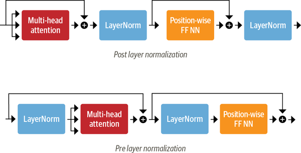
向 Transformer Encoder/Decoder 中添加 layer normalization 目前共有两种做法:
- Post layer normalization:Transformer 论文中使用的方式,将 layer normalization 放在 skip connections 之间。 但是因为梯度可能会发散,这种做法很难训练,通常还需要结合学习率预热 (learning rate warm-up) 等技巧;
- Pre layer normalization:这是目前主流的做法,将 layer normalization 放置于 skip connections 的范围内。这种做法通常训练过程会更加稳定,并且不需要任何学习率预热。
下面我们采用第二种方式来构建 Transformer Encoder 层:
class TransformerEncoderLayer(nn.Module):
    def __init__(self, config):
        super().__init__()
        self.layer_norm_1 = nn.LayerNorm(config.hidden_size)
        self.layer_norm_2 = nn.LayerNorm(config.hidden_size)
        self.attention = MultiHeadAttention(config)
        self.feed_forward = FeedForward(config)

    def forward(self, x, mask=None):
        # Apply layer normalization and then copy input into query, key, value
        hidden_state = self.layer_norm_1(x)
        # Apply attention with a skip connection
        x = x + self.attention(hidden_state, hidden_state, hidden_state, mask=mask)
        # Apply feed-forward layer with a skip connection
        x = x + self.feed_forward(self.layer_norm_2(x))
        return x
同样地,我们将之前构建的输入送入到该层中进行测试:
encoder_layer = TransformerEncoderLayer(config)
print(inputs_embeds.shape)
print(encoder_layer(inputs_embeds).size())
torch.Size([1, 5, 768])
torch.Size([1, 5, 768])
至此,我们就使用 Pytorch 从头构建出了一个 Transformer Encoder 层。
但是,由于 Multi-head Attention 无法捕获 token 之间的位置信息,因此我们还需要使用 Positional Embeddings 向模型中添加 token 位置信息。
Positional Embeddings
Positional Embeddings 基于一个简单但有效的想法:使用与位置相关的值模式来增强 token 嵌入表示。最简单的方法就是让模型自动学习位置嵌入,尤其是在预训练数据集足够大的情况下。下面我们以这种方式创建一个自定义的 Embeddings 模块,它同时将 token 和位置映射到嵌入式表示,最终的输出是两个嵌入式表示的和:
class Embeddings(nn.Module):
    def __init__(self, config):
        super().__init__()
        self.token_embeddings = nn.Embedding(config.vocab_size,
                                             config.hidden_size)
        self.position_embeddings = nn.Embedding(config.max_position_embeddings,
                                                config.hidden_size)
        self.layer_norm = nn.LayerNorm(config.hidden_size, eps=1e-12)
        self.dropout = nn.Dropout()

    def forward(self, input_ids):
        # Create position IDs for input sequence
        seq_length = input_ids.size(1)
        position_ids = torch.arange(seq_length, dtype=torch.long).unsqueeze(0)
        # Create token and position embeddings
        token_embeddings = self.token_embeddings(input_ids)
        position_embeddings = self.position_embeddings(position_ids)
        # Combine token and position embeddings
        embeddings = token_embeddings + position_embeddings
        embeddings = self.layer_norm(embeddings)
        embeddings = self.dropout(embeddings)
        return embeddings

embedding_layer = Embeddings(config)
print(embedding_layer(inputs.input_ids).size())
torch.Size([1, 5, 768])
除此以外,Positional Embeddings 还有一些替代方案:
绝对位置表示:使用由调制的正弦和余弦信号组成的静态模式来编码 token 位置。 当没有大量训练数据可用时,这种方法尤其有效;
相对位置表示:在生成某个 token 的 embedding 时,一般距离它近的 token 更为重要,因此相对位置表示编码 token 之间的相对位置。这种表示无法通过简单地引入嵌入层来完成,因为每个 token 的相对嵌入会根据我们关注的序列的位置而变化,这需要在模型层面对注意力机制进行修改,例如 DeBERTa 等模型。
下面我们将所有这些层结合起来构建完整的 Transformer encoder:
class TransformerEncoder(nn.Module):
    def __init__(self, config):
        super().__init__()
        self.embeddings = Embeddings(config)
        self.layers = nn.ModuleList([TransformerEncoderLayer(config)
                                     for _ in range(config.num_hidden_layers)])

    def forward(self, x, mask=None):
        x = self.embeddings(x)
        for layer in self.layers:
            x = layer(x, mask=mask)
        return x
同样地,我们对该层进行简单的测试:
encoder = TransformerEncoder(config)
print(encoder(inputs.input_ids).size())
torch.Size([1, 5, 768])
Transformer Decoder
Transformer Decoder 与 Encoder 最大的不同在于 Decoder 有两个注意力子层,如下图所示:
Masked multi-head self-attention layer:确保我们在每个时间步生成的 token 仅基于过去的输出和当前预测的 token,否则 Decoder 就可以在训练期间直接看到翻译答案,相当于作弊了。
Encoder-decoder attention layer:以解码器的中间表示作为 queries,对 encoder stack 的输出 key 和 value 向量执行 Multi-head Attention。通过这种方式,Encoder-Decoder Attention Layer 就可以学习到如何关联来自两个不同序列的 token,例如两种不同的语言。 解码器可以访问每个 block 中 Encoder 的 keys 和 values。
与 Encoder 中的 Mask 不同,Decoder 的 Mask 是一个下三角矩阵:
seq_len = inputs.input_ids.size(-1)
mask = torch.tril(torch.ones(seq_len, seq_len)).unsqueeze(0)
print(mask[0])
tensor([[1., 0., 0., 0., 0.],
        [1., 1., 0., 0., 0.],
        [1., 1., 1., 0., 0.],
        [1., 1., 1., 1., 0.],
        [1., 1., 1., 1., 1.]])
这里我们使用 PyTorch 自带的 tril() 函数来创建下三角矩阵,然后同样地,通过 Tensor.masked_fill() 将所有零替换为负无穷大来防止注意力头看到未来的 token 而造成信息泄露:
scores.masked_fill(mask == 0, -float("inf"))
tensor([[[26.8082,    -inf,    -inf,    -inf,    -inf],
         [-0.6981, 26.9043,    -inf,    -inf,    -inf],
         [-2.3190,  1.2928, 27.8710,    -inf,    -inf],
         [-0.5897,  0.3497, -0.3807, 27.5488,    -inf],
         [ 0.5275,  2.0493, -0.4869,  1.6100, 29.0893]]],
       grad_fn=<MaskedFillBackward0>)
本文的重点在于实现 Encoder,因此对于 Decoder 只做简单的介绍,如果你想更深入的了解可以参考 Andrej Karpathy 实现的 minGPT。
参考
[1] 《Attention is All You Need》浅读(简介+代码)
[2] 《Natural Language Processing with Transformers》
附录
本文核心代码整理于 Github:
https://gist.github.com/jsksxs360/3ae3b176352fa78a4fca39fff0ffe648